
Demand Forecasting with Machine Learning: From Azure ML to Databricks
Better demand forecasts start before model training. Explore how clean data, strong baselines and the right Azure ML or Databricks tools can help your team reduce stockouts, manage excess inventory and build forecasts planners can trust.
Demand forecasting with machine learning predicts future demand from historical sales, market trends and outside factors such as weather, promotions and holidays. The model learns patterns that fixed formulas miss. McKinsey finds that AI-driven forecasting in supply chain management can reduce errors by 20 to 50 percent. The M5 forecasting competition was won by a student with very limited forecasting background. The winning entry was pure machine learning with no statistical components.
For energy, medtech and restaurant leaders, that means this work doesn’t need a research lab. A capable analytics team can do it. The payoff depends on the data under the model and the platform features you build on. On Azure Machine Learning and Databricks, several forecasting tools are still in preview, and one is on its way out.
Machine Learning Learns from Every Product and Location at Once
Machine learning improves demand forecasting by training one model across thousands of product and location series. It uses sales history plus outside signals instead of fitting a separate formula to each item. IBM defines demand forecasting as “the systematic process within supply chain management that uses historical data, market trends and external economic indicators for demand planning.”

Traditional statistical tools work one series at a time. A moving average or ARIMA model projects a single product’s past sales forward. A machine learning model sees the whole portfolio. It can learn that a price cut on one item pulls sales from another, or that a hot weekend lifts demand across a region.
Patterns from high-volume items also help forecast slow movers with sparse history. That matters for a medtech catalog or a restaurant menu with a long tail of low-volume items.
Historical sales remain the foundation. For a restaurant group, that means ingredient usage by location and day. For a medtech manufacturer, it means units shipped by SKU and account. For an energy company, it might be fuel or parts consumption by site. If that record is wrong, no algorithm will rescue the forecast.
Inventory Distortion Cost Retailers $1.7 Trillion in 2026
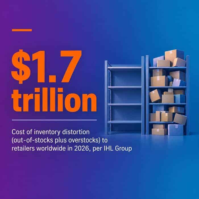
Inventory distortion, meaning out-of-stocks plus overstocks, cost retailers worldwide $1.7 trillion in 2026, according to IHL Group. That equals 6.2% of global retail sales, down from 10.4% in 2021. IHL attributes $690.9 billion of it to empty shelves alone.
The mechanics carry over to any business that stocks product. Forecast too high and capital sits in warehouses, walk-in coolers or consignment inventory. Forecast too low and you lose the sale, pay for rush replenishment, or leave a customer waiting.
The stakes differ by industry. Perishable ingredients spoil when a restaurant overorders. A missing implant or instrument set can push back a scheduled procedure. In energy, a shortfall in fuel or critical spare parts can idle equipment.
Trusted forecasts also make supply chains more resilient. Planners can spend their time on real exceptions, such as a supplier disruption or a storm, instead of rebuilding numbers by hand.
Statistical Methods Set the Baseline and Machine Learning Beats It
Traditional forecasting methods still earn a place in every project, because they give you the benchmark a machine learning model has to beat. Qualitative methods rely on judgment from sales teams, planners or field staff. Quantitative methods apply statistics to past sales, including moving averages, Naive forecasts that repeat the last value, ARIMA and exponential smoothing.
Machine learning adds two abilities. It uses many causal inputs at once, and it forecasts at a fine grain, such as every item in every store. The table compares the two approaches on the points that matter for a build decision.
| Factor | Traditional Methods | Machine Learning |
|---|---|---|
| Typical inputs | Past sales of one series | Sales plus causal features |
| Unit of modeling | One model per series | One model across many series |
| Causal factors | Few or none | Many at once |
| Fine-grained forecasts | Slow to scale | Built for store-item scale |
| Explainability | High | Moderate, needs tooling |
| Setup effort | Low | Higher data and engineering effort |
| Best fit | Baselines and stable demand | Promotions, many SKUs, volatile demand |
Keep both in your toolkit. A machine learning model that cannot beat a seasonal naive forecast on held-out data isn’t ready for production, however sophisticated it looks.
Start with a Seasonal Naive Baseline, Then Try LightGBM
Start with a simple baseline, then add a gradient-boosted tree model. Hold deep learning back until scale justifies it. The M5 Accuracy competition supports that order. In M5, LightGBM showed superior forecasting performance over all other alternatives, and practically all of the top 50 entries used it.
Gradient-boosted trees such as LightGBM and XGBoost suit demand data because it is tabular and feature-rich. Each row can carry the date, location, price, promotion flag, holiday and weather alongside lagged sales. Trees handle that mix with little manual tuning.
| Method | Role | Use When |
|---|---|---|
| Seasonal Naive | Baseline to beat | Every project |
| Moving average | Simple smoothing | Stable, low-volume demand |
| ARIMA / SARIMA | Statistical benchmark | Clear trend or seasonality |
| Exponential smoothing | Statistical benchmark | Few series, steady patterns |
| Linear regression | Interpretable causal model | A few well-understood drivers |
| LightGBM / XGBoost | Primary ML model | Many series and features |
| Deep learning (TCN, DeepAR) | Advanced option | Very large series counts |
| Time-series foundation model | Fast first forecast | Quick baseline from SQL |
Seasonality and variability decide which baseline is hard to beat. Demand with a strong weekly or annual cycle, such as restaurant traffic, often suits SARIMA (seasonal ARIMA) or exponential smoothing. Intermittent demand, common for medtech spare parts or specialized energy equipment, has many zero periods. Every method struggles there. Trees pull ahead on promotion-heavy or weather-sensitive demand, because they learn from those drivers directly.
Deep learning with Python models such as temporal convolutional networks (TCN) and DeepAR can capture complex patterns across very large collections of series. They cost more to train and are harder to explain to a planner. A time-series foundation model is pretrained on many series and can forecast without task-specific training. That makes it a fast way to get a first number.
Clean Sales History Matters More Than the Algorithm You Pick
Clean, governed sales history at your forecast grain drives quality more than any algorithm choice. Budget for it ahead of model tuning. Check four dimensions before modeling. Volume means enough history to see repeated seasonal cycles. Granularity means records at the forecast grain, such as item by location by day.
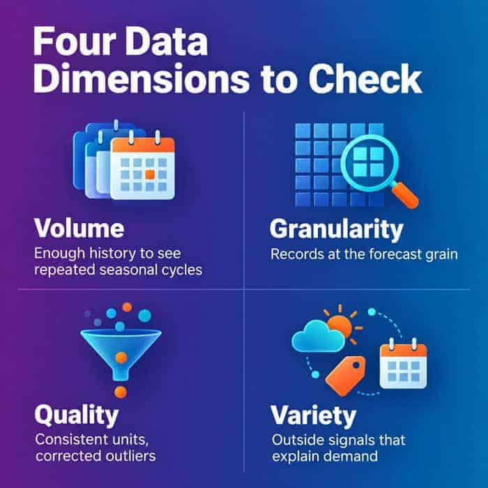
Quality means consistent units, corrected outliers, and missing periods filled or flagged. Variety means the outside signals that explain demand. Use this checklist to assemble the inputs for a first model.
One rule catches teams off guard. Azure Machine Learning’s AutoML regression forecasting models assume every feature you provide is known into the future, at least up to the forecast horizon. Suppose you train on actual weather but can only supply a forecast of next week’s weather. The model will look better in testing than it performs in production. Include only inputs you will reliably have in advance.
Social media signals and economic indicators can help with longer-horizon or category-level planning. They are rarely available ahead of time at the store-item level. Treat them as experiments once the core model works.
Seven Steps to Build Demand Forecasting with Machine Learning
Fix the business goal and baseline metric before anyone trains a model. Many organizations skip that discipline. A Gartner survey of 120 supply chain leaders who had deployed AI found only 23% of supply chain organizations had a formal AI strategy. It was fielded from December 2024 to January 2025.
Azure ML and Databricks Both Scale Forecasts, with Different Caveats
Azure Machine Learning and Databricks can both forecast thousands of series at a fine grain. They package the work differently and carry different preview and deprecation risks.
| Capability | Azure Machine Learning | Databricks |
|---|---|---|
| Automated forecasting | AutoML forecasting | Serverless forecasting |
| Classical models | ARIMA(X) and Exponential Smoothing | Prophet and Auto-ARIMA (classic AutoML) |
| Deep learning | TCN | DeepAR |
| Scale pattern | Many models | Per store-item accelerator |
| Status to watch | Distributed TCN training in preview | Classic AutoML deprecated |
Azure Machine Learning Builds Baselines into AutoML
Azure ML’s AutoML forecasting tests classical baselines and machine learning models in the same run. That builds the baseline-first discipline into the tool. Microsoft documents that AutoML tunes Exponential Smoothing and ARIMA(X) by grid search. Its model recommendation service tunes tree and linear models dynamically. Naive-family models aren’t tuned at all, which suits a benchmark.
For scale, Azure ML supports “many models” forecasting. Distributed training and model search for TCN deep learning models remain a preview feature. For organizations standardized on Microsoft, demand forecasting with Azure Machine Learning keeps data, models and security policies in a familiar environment.
Databricks Offers an Accelerator, Serverless Forecasting and SQL
Databricks, a data intelligence platform for enterprise analytics, gives teams three routes to a forecast. They differ sharply in maturity. The Demand Forecasting Solution Accelerator builds a forecast for each store-item combination on distributed compute. It updates forecasts as new sales data arrives and runs in Python or R.
Serverless forecasting is the newer automated option. It adds the DeepAR deep learning algorithm, Unity Catalog registration, custom train, validation and test splits, and per-series weights. Unity Catalog puts the model under the same governance layer as your data.
The third route needs no Python. Databricks SQL’s ai_forecast() version 2 runs on a pretrained time-series foundation model. It supports holidays, covariates and non-negative forecasts. It requires a Pro or Serverless SQL warehouse plus enrollment in the Predictive AI Functions preview. It launched as one of five Predictive AI Functions, alongside ai_top_drivers, ai_detect_anomalies, ai_predict_value and ai_predict_class.
Preview and Deprecation Status Is the Real Platform Risk
The biggest platform risk is building production work on a feature still in preview or already scheduled for removal. Databricks states that its AutoML “is deprecated and will be removed in the next major Databricks Runtime ML version.” It recommends the Data Science Agent, currently in Beta, or AI Functions instead.
On classic compute, Databricks AutoML forecasting runs Prophet and Auto-ARIMA, and its experiments stop after 120 minutes by default. Any pipeline built on it needs a migration plan now.
Preview features carry their own risk. The earlier version of ai_forecast() was itself a Public Preview that required Databricks SQL 2024.35 or later. Use preview tools for prototypes and quick baselines. Put generally available features under anything a planner depends on daily. Build with purpose, not patchwork.
M5 Results Show What Good Forecast Accuracy Looks Like
The M5 competition is the clearest public evidence that machine learning beats strong statistical benchmarks on demand data, and it gives leaders realistic targets. In the M5 Accuracy competition, every one of the top 50 entries beat the best of 24 benchmarks by more than 14%. The M5 winner beat it by 22.4%. It was the first M competition in which all the top-performing methods were pure machine learning.
Those gains are measured against the best benchmark, not against a neglected spreadsheet. If your current process is weaker than a good statistical baseline, your first improvement may come from putting a disciplined baseline in place.
Industry evidence points the same way. McKinsey reports that AI-driven forecasting can cut lost sales and product unavailability by up to 65%. Gartner predicts that 70% of large organizations will use AI-based forecasting to predict future demand by 2030.
Set your own target in business terms. A percentage reduction in error against your baseline, tied to stockouts avoided or inventory released, is the number a CFO will fund.
Measure Accuracy Every Cycle and Keep Planners in the Loop
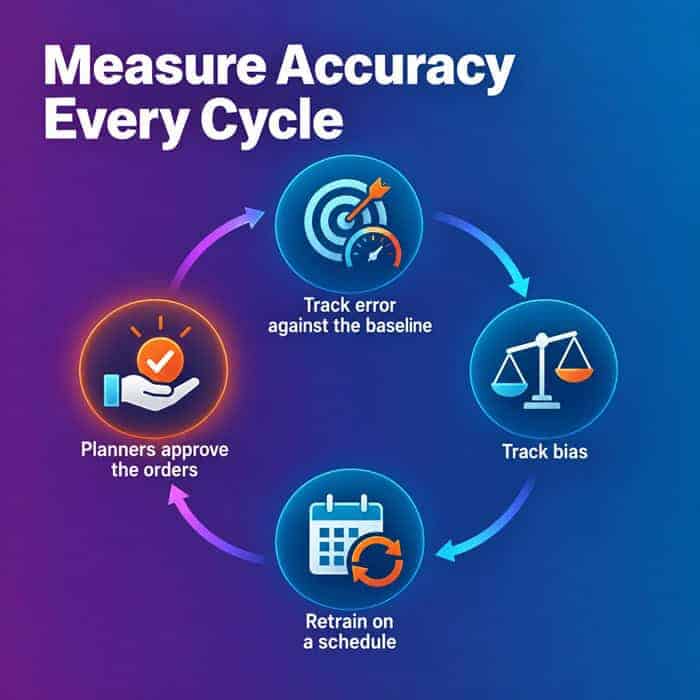
Forecast accuracy decays after launch as menus, product lines, prices and customer behavior change, so monitoring belongs in the design from day one. Track error against the baseline every planning cycle. Mean absolute percentage error (MAPE) is common, and weighted absolute percentage error (WAPE) reads better when many items sell in small quantities.
Track bias too. A model that consistently overforecasts will quietly inflate inventory even when its average error looks fine.
Retrain on a schedule as new sales arrive, rather than waiting for someone to notice a problem. Watch for structural breaks, such as a new store format, a product recall or a plant turnaround, that make older history less relevant.
Keep people accountable for the decisions. Gartner predicts that by 2030 only 5% of organizations using supply chain planning automation will make at least 10% of their planning decisions autonomously. The practical design is intelligent automation that produces the forecast and flags exceptions, with planners approving the orders. That gives you less guesswork without giving up judgment.
Ready to get started? Talk to a Smartbridge expert about scoping your forecasting pilot.